Network Theory - Six Degrees of Separation

February 6, 2022

Intro

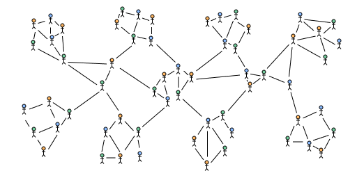
It is often said that all pairs of individuals in the world can reach each other in a chain of no more than six acquaintances. This idea of six degrees of separation can be represented as a property of a mathematical network called the small world property and has been shown to be true for models that are built to match characteristics of social networks in the real world.

Network theory is a branch of applied mathematics interested in the study of the structure of graphs where the nodes and edges represent objects and relationships for example friends in a social group, flights between airports or websites on the internet.

Small world property

How could we define a small world mathematically? If we take any pair of random individuals and find the minimum number of acquaintances in a chain starting from one person to the other then we can equivalently represent this as the shortest path (called a geodesic) between two nodes in a social network where the nodes represent individuals and the edges represent being acquainted with each other.

A small world can then be defined as a network where the average shortest path length $\ell$ grows slowly compared to the number of nodes in the network $n$ . More formally:

\ell = O\bigl(log(n)\bigr) \quad \text{ as } n\to\infin

In other words, for sufficiently large $n$ , the degrees of separation grows at most logarithmically.

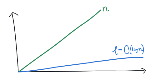small-world-asymptotic Asymptotic growth of $\ell$ relative to $n$ in a small world

Milgram experiment

In the 1960s an American social psychologist named Stanley Milgram conducted an experiment with a team from Harvard to find $\ell$ in the US. The experiment is summarized as follows:

Begin by delivering packages to selected start individuals in the states of Nebraska and Kansas. The package contained a letter with the official Harvard crest explaining the experiment and a list to record the recipient's own name.
The recipient was instructed to attempt to forward the letter to a target in Boston, either directly if they knew them on a first name basis, or to someone they believed would be socially closer to the target.
After repeating the previous step and the target successfully received the letter, check the list of names to analyze the path taken through the social network.

In one of these experiments 18 out of 96 letters successfully completed a journey from the start to the target. Out of these paths, the average path length was 5.9 which provided early empirical evidence supporting the theory of "six degrees of separation".

Erdős–Rényi model

The Erdős–Rényi model $G(n,p)$ is a simple random graph model for generating a network. In this model we have a fixed number of vertices $n$ and each of the $n \choose 2$ possible edges between pairs of vertices is present with probability $p$ independently. This model has the small world property, in fact as $n$ grows large, almost all paths have the same shortest length.

An intuition for this can be thought of by considering a single node and the expected number of neighbours it can reach within a certain distance $x$ . The average number of neighbours of a node in $G(n,p)$ is $\langle k \rangle = (n-1)p$ as there are $n - 1$ possible edges to nodes excluding yourself each present with probability $p$ . For large $n$ at a distance of $x$ we can then roughly reach $(n-1)^xp^x$ nodes.

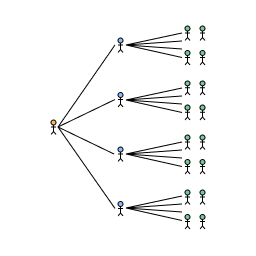erdos-renyi-friends Number of friends reachable in $G(n,p)$ at a distance of $x$

To reach all nodes at the shortest distance $\ell$ we then have:

\begin{align*} && (n-1)^\ell p^\ell &\approx n \\ \implies \qquad && \langle k \rangle ^\ell &\approx n\\ \implies \qquad && \ell &\approx log_{\langle k \rangle}(n) \\ \implies \qquad && \ell &\approx O\bigl(log(n)\bigr) \end{align*}

However, the Erdős–Rényi model does not share other characteristics of real world networks.

The degree distribution of a network is the probability distribution of the degree (number of edges of a node) over the whole network. For $G(n,p)$ the degree distribution is binomial which does not match observations of most networks in the real world which typically have a larger variance of degrees with many nodes having a low degree and a small number of nodes acting as hubs with a large degree.

The clustering coefficient of a network is a measure of how much nodes tend to group together. A version of it can be defined as the ratio between the number of triangles (a triplet of nodes with all three possible edges between them present) and the number of connected triplets (a triplet of nodes with only two edges between them) in the network. For $G(n,p)$ the expected clustering coefficient is $p$ as $n$ grows large which is low for small $p$ . This also does not match observations of most networks in the real world which typically exhibit a high clustering coefficient.

Watts-Strogatz model

The Watts-Strogatz model followed the Erdős–Rényi model and was designed to achieve both a high clustering coefficient and the small world property via an edge rewiring mechanism.

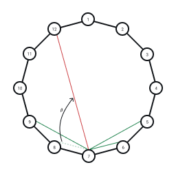
We start with an initial ring lattice with $N$ nodes with each node having degree $K$ with edges to the nearest $\frac{K}{2}$ nodes to the left and the nearest $\frac{K}{2}$ nodes to the right. Here we demonstrate $N=12$ and $K=4$ :

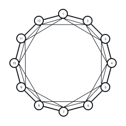watts-strogatz-ring Initial ring lattice with $\frac{NK}{2}$ edges

For each node we consider the $\frac{K}{2}$ edges to the nodes to the left and with probability $\beta$ rewire the edge randomly to another node that does not already have an edge to the current node:

watts-strogatz-rewire Rewiring of an edge with probability $\beta$ in the Watts-Strogatz model

Repeating this rewiring step over all nodes we complete the random graph:

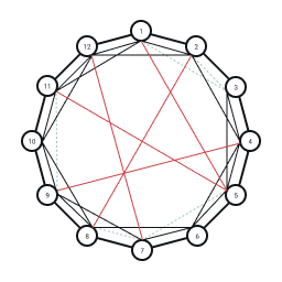watts-strogatz-finish Completed random graph generated from rewiring process

The rewired edges can be thought of as "shortcuts" or "wormholes" through the network and significantly decrease the average shortest path length $\ell$ . It makes sense then that as $\beta$ increases, $\ell$ rapidly approaches its limiting value $\ell \approx \frac{\ln N}{\ln K}$ at $\beta = 1$ and the network has the small world property.

The clustering coefficient in the initial ring lattice is high as the edges to close neighbours means that neighbours tend to form cliques. This drops as $\beta \to 1$ and the edges become completely random but in the intermediate values of $\beta$ we achieve both a high clustering coefficient and the small world property.

The main drawback of the model is the unrealistic homogeneity of the degree distribution. In the initial ring lattice all nodes have degree $K$ and after rewiring the degree distribution is still centred around $K$ . The rewiring process also only works on a fixed set of nodes and so cannot model a growth process of adding new nodes to the network.

Barabási–Albert model

The Barabási–Albert model uses a preferential attachment mechanism in order to achieve both a heterogeneous degree distribution and the small world property.

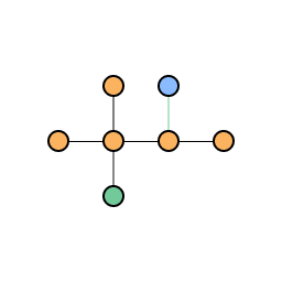
We start with an initial set of $m_0$ nodes and edges such that the graph is connected and choose $m <= m_0$ such that at each step we add a new node to the network with $m$ edges to existing nodes in the network. Here we demonstrate the preferential attachment process with $m_0 = 5$ and $m = 1$ .

barabasi-albert-initial Initial network with $m_0$ = 5

When adding a new node to the network we choose $m$ existing nodes to add edges to. The probability $p_i$ that we attach to an existing node $i$ is weighted by its degree $k_i$ using the distribution $p_i = \frac{k_i}{\sum_j{k_j}}$ . Hence, highly linked nodes are "preferred" and more likely to accumulate more edges.

barabasi-albert-one-step Network after one step of growth with $m = 1$

Repeating this process for a second step we add a second new node and connect it to another existing node weighted by its degree:

barabasi-albert-two-steps Network after two steps of growth with $m = 1$

We repeat this process until we reach the desired network size:

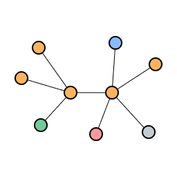barabasi-albert-final Final network after repeating growth by preferential attachment

Notice that preferential attachment leads to hub and spoke network with a small number of highly connected hub nodes serving as gateways to reach other nodes in the network where there are many spoke nodes with a small number of edges. This can also be thought of as "the rich get richer and the poor get poorer" effect where well established nodes continue to get richer in edge count whereas newer nodes struggle to gain new edges.

The degree distribution in fact follows a power law distribution which is known as a scale free network.

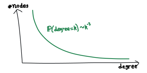barabasi-albert-power-law Power law degree distribution

The hub and spoke structure leads to a low average shortest path length with $\ell \approx \frac{log N}{log log N}$ asymptotically so the Barabási–Albert model has the small world property. Preferential growth allows simulating network growth and produces a similar degree distribution to real world examples such as airport hub and spoke networks where major hub cities are more likely to attract new flights rather than smaller less desirable locations.

Unfortunately, the clustering coefficient in the Barabási–Albert model also follows a power law and therefore is small when the network is large.

Conclusion

We have defined mathematically what it means for a network to be a small world and introduced three models which all exhibit the small world property with their own drawbacks when comparing to real world networks. Hopefully, this provides more insight into the phrase "six degrees of separation", in fact with modern technology perhaps this should be closer to three and a half!